Quickstart

This walkthrough goes from nothing to a hotspot forecast in a few minutes, using synthetic data so you can run it as is. Every step is explained in depth in the user guide.

1. A study area

Predspot needs the boundary of the region you are studying as a GeoDataFrame with a CRS. The easiest way is to fetch it from OpenStreetMap (osmnx is installed with Predspot):

from predspot import load_study_area

study_area = load_study_area("Natal, Rio Grande do Norte, Brazil")

Any other source works too — a shapefile or GeoJSON read with geopandas.read_file, or a simple box:

import geopandas as gpd
from shapely.geometry import box

study_area = gpd.GeoDataFrame(geometry=[box(-35.30, -5.90, -35.20, -5.80)], crs="EPSG:4326")

2. Crime events

Your data must be a pandas DataFrame with four columns:

Column	Meaning
tag	Crime type (any string)
t	Timestamp (anything pandas.to_datetime understands)
lon, lat	Coordinates in WGS84 degrees

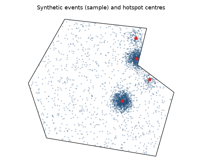
No data at hand? Generate realistic synthetic events inside the study area:

from predspot import generate_crimes

crimes = generate_crimes(study_area, n_events=5000, n_hotspots=4,
                         start="2019-01-01", end="2020-12-31", seed=0)
crimes.head()

Wrap both in a Dataset:

from predspot import Dataset

dataset = Dataset(crimes, study_area)
dataset.plot()   # study area + a sample of events

3. Build and fit a pipeline

A PredictionPipeline chains a spatio-temporal mapping, a feature extraction step and a scikit-learn estimator:

from sklearn.ensemble import RandomForestRegressor

from predspot import PredictionPipeline, PandasFeatureUnion
from predspot.crime_mapping import KDE, create_gridpoints
from predspot.feature_engineering import Seasonality, Trend, Diff

grid = create_gridpoints(study_area, resolution=1)   # points every 1 km

pipeline = PredictionPipeline(
    mapping=KDE(tfreq="M", grid=grid),               # monthly density per point
    fextraction=PandasFeatureUnion([
        ("seasonal", Seasonality(lags=6)),
        ("trend", Trend(lags=6)),
        ("diff", Diff(lags=6)),
    ]),
    estimator=RandomForestRegressor(n_estimators=100, random_state=0),
    random_state=0,
)
pipeline.fit(dataset)

build_default_pipeline builds exactly this kind of pipeline (with scaling and feature selection) in one call.

4. Evaluate and forecast

pipeline.evaluate("r2", cv=3)     # one score per time series fold
forecast = pipeline.predict()     # DataFrame indexed by (t, places)

forecast holds the predicted density for the month after the last observed one, for every grid point. Join it with the grid to map it:

hot = pipeline.grid.join(forecast.droplevel("t"))
hot.plot(column="crime_density", cmap="magma", markersize=12, legend=True)

Calling predict() again forecasts the following month, and so on — each forecast is appended to the series and the features are recomputed.

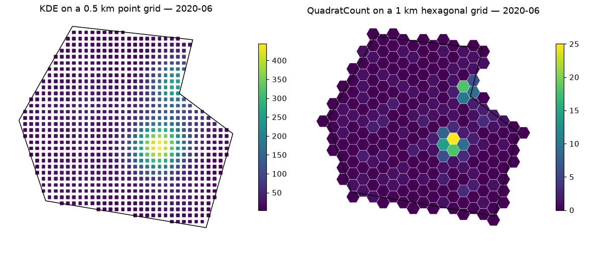
5. Prefer counts on hexagons?

Swap the mapping and the grid; everything else stays the same:

from predspot.crime_mapping import QuadratCount, create_gridhexagonal

mapping = QuadratCount(tfreq="W", grid=create_gridhexagonal(study_area, resolution=1))

The same month mapped with KDE on a point grid (left) and with event counts on a hexagonal grid (right).