Data and study areas
Crime events
Predspot works with point events: one row per crime with a type, a timestamp and a location. The input is a plain pandas DataFrame with the columns below; extra columns are kept and ignored.
| Column | Type | Notes |
|---|---|---|
tag |
str | Crime type. Filter on it to model one type at a time. |
t |
datetime-like | Parsed with pandas.to_datetime. Timezone-naive local time is the simplest. |
lon |
float | Longitude in WGS84 degrees (EPSG:4326). |
lat |
float | Latitude in WGS84 degrees. |
import pandas as pd

crimes = pd.read_csv("crimes.csv", parse_dates=["t"])
crimes = crimes[crimes["tag"] == "robbery"]
Study area
The study area is a GeoDataFrame with one or more polygons and a CRS. It bounds the grids and is used for plotting; events outside it are not removed, but grid cells are only created where they intersect it.
from predspot import load_study_area

study_area = load_study_area("Natal, Rio Grande do Norte, Brazil")
load_study_area geocodes the
place with osmnx (Nominatim) and returns
its administrative boundary. Be specific — add the state and country —
so that the first match is the boundary you want; which_result lets you
pick another match. osmnx is installed with Predspot.
Any CRS is accepted; grids are re-projected to it.
The Dataset object
from predspot import Dataset

dataset = Dataset(crimes, study_area)
dataset                      # summary with counts per tag
dataset.crimes               # GeoDataFrame of points (WGS84), `t` parsed
dataset.study_area
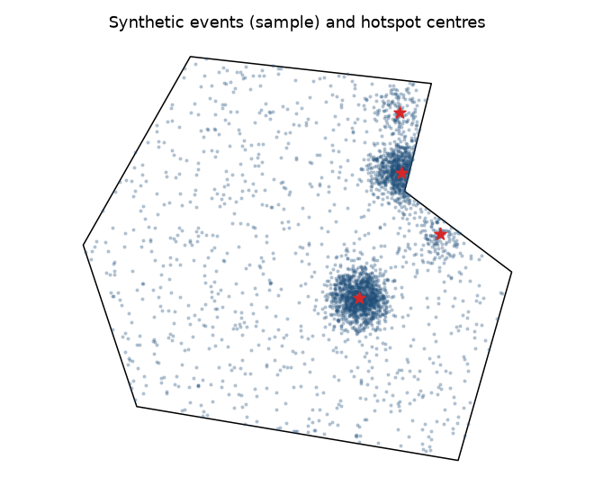
dataset.plot(crime_samples=2000)
train, test = dataset.train_test_split(test_size=0.25, random_state=0)
Dataset validates the inputs and never modifies the DataFrame you pass in.
Synthetic data
generate_crimes produces events with
the structure real crime data tends to have, inside any study area:
- space:
n_hotspotsGaussian clusters (centres drawn inside the area, spreadhotspot_sd_km) holding ahotspot_shareof the events, plus a uniform background; - time: an intensity combining a linear
trend, an annual cycle (annual_amplitude,annual_peak_month), aweekly_profile(Monday to Sunday) and anhourly_profile(0-23 h). Timestamps are sampled by thinning, so the patterns are exact in expectation.
from predspot import generate_crimes

crimes, hotspots = generate_crimes(
    study_area, n_events=8000, n_hotspots=4, hotspot_sd_km=0.6,
    start="2019-01-01", end="2020-12-31",
    trend=0.3, annual_amplitude=0.3, annual_peak_month=12,
    tags={"robbery": 0.6, "burglary": 0.4},
    seed=7, return_hotspots=True,
)
hotspots is a GeoDataFrame with the centre, spread and share of each
hotspot — handy to check what a model recovers. Set n_hotspots=0 for a
uniform map, weekly_profile=None / hourly_profile=None to switch those
patterns off, and a seed for reproducibility.