Grids and spatio-temporal mapping¶

Mapping turns raw events into the spatio-temporal series: one value per place and period. It is the step that defines what "hotspot" means in your analysis.

Grids¶

All grid functions take the study area and a resolution in kilometres, and return a GeoDataFrame with geometry, lon, lat columns and an index named places. Only cells intersecting the study area are kept.

Function	Cells	Pairs with
`create_gridpoints`	points spaced `resolution` km apart	`KDE` (default)
`create_gridhexagonal`	hexagons with the area of a `resolution` km square	`QuadratCount`
`create_gridsquares`	squares of side `resolution` km	`QuadratCount`

from predspot.crime_mapping import create_gridpoints, create_gridhexagonal

points = create_gridpoints(study_area, resolution=0.5)
hexes = create_gridhexagonal(study_area, resolution=1)
hexes.plot(edgecolor="white")

Choosing a resolution is a trade-off: finer grids give more spatial detail but more places to model (and, for KDE, more points to evaluate); the original work used 250 m to 1 km for city-scale studies. Hexagons are preferable to squares for counts because every neighbour is at the same distance.

Time frequency¶

tfreq sets the period: "D" (daily), "W" (weekly, Sunday-ending) or "M" (monthly, month-end labels). Periods without events are kept with zeros, and start_time / end_time can pad the series.

KDE¶

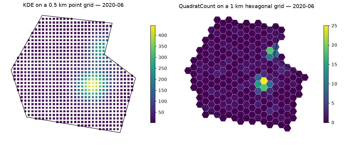
KDE fits a Gaussian kernel density estimate (scipy.stats.gaussian_kde) to the event coordinates of each period and evaluates it at the grid points. The result is a smooth density surface — the classic hotspot map.

from predspot.crime_mapping import KDE

mapping = KDE(tfreq="M", grid=points, bandwidth="silverman")
stseries = mapping.fit_transform(dataset.crimes)
stseries.head()

t           places
2019-01-31  0         12.31
            1         14.02
            ...
Name: crime_density, dtype: float64

bandwidth can be "silverman", "scott" or a number. With a rule of thumb the factor is estimated on the first period with at least three events and then held fixed, so that densities are comparable across time; mapping.factor tells you what was used. Periods with fewer than three events map to zero.

QuadratCount¶

QuadratCount counts the events that fall inside each polygonal cell. Counts are easier to interpret than densities (they are numbers of crimes) and lend themselves to count models, at the price of a blockier map and sensitivity to how the grid is laid out.

from predspot.crime_mapping import QuadratCount

mapping = QuadratCount(tfreq="W", grid=hexes)
stseries = mapping.fit_transform(dataset.crimes)
stseries.groupby("t").sum()      # events per week

Writing your own mapping¶

Subclass SpatioTemporalMapping and implement fit_grid(data_points), which receives the events of one period and returns a {place: value} dict. The base class handles the time splitting, empty periods and the assembly of the series, so your mapping is immediately usable in a PredictionPipeline.

from predspot.crime_mapping import SpatioTemporalMapping

class NearestCount(SpatioTemporalMapping):
    """Number of events closer than 300 m to each grid point."""

    def fit_grid(self, data_points):
        pts = data_points.to_crs(self._grid.estimate_utm_crs())
        grid = self._grid.to_crs(pts.crs)
        return {p: int(pts.distance(geom).lt(300).sum())
                for p, geom in grid.geometry.items()}